It is fairly easy to construct a retrospective efficiency rating. Take the efficiencies for each game, correct for location and rest, and then solve using an OLS regression for each team’s true efficiency rating. Nice and neat.
However, how should a predictive rating work? The best approach would be to adjust for what players are playing and when, but in this investigation I’ll restrict myself to team-level data. If I have the same data (efficiencies for each game), how would I best predict game n+1?
The obvious approach is to attack the issue from a Bayesian perspective, so I shall.
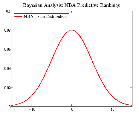
Suppose we assume that the teams are distributed based on a normal distribution curve with mean 0. That’s a pretty good assumption; the overall results tend to look like the famous bell curve. Lots of teams close to average; a few outliers. We’ll roll with that assumption.
Assume, also, that each team’s performances are a random sampling drawn from a normal distribution around that team’s true efficiency level. This is not necessarily as good an assumption–if Lebron were out 35 games, those games are not taken from the same sample that the games WITH Lebron are drawn from. Also, teams tend to pull their starters in blowouts, leading to results that show “playing to the level of the opponent”. Dean Oliver talked about this back in 1997, discussing removing the covariance of team offense and defense. Furthermore, teams make trades during the season; some help the team’s current level, some hurt. Finally, opponents also are having the same issues that make opponent adjustments (assuming the opponent has the same true level all year) rather dicey.
Nevertheless, for this first exercise in Bayesian inference, I will make the assumption that the sampled performances are from a normal distribution.
Okay, so we have a prior distribution–the overall league distribution, centered on 0. Standard deviation is right around 5 (I just checked the average efficiency differentials for the 30 teams, and the standard deviation was about 5).
Cool!
Now the hard part: we have lots of observations of how teams performed in given games. Since this is a predictive rating, we are considering the possibility that older samples are not as good as more recent samples (i.e. there is a transformation function applied between each game). How do we incorporate these observations in a Bayesian framework?
Well, we need some sort of “standard error” to associate with each game’s observation. In general, the team’s performance over the season (adjusted for opponent, rest, & location) have a standard deviation of about 12.5, but that includes the variation that we are trying to adjust for (the change through the season). I’ll use 12 as the starting point per game.
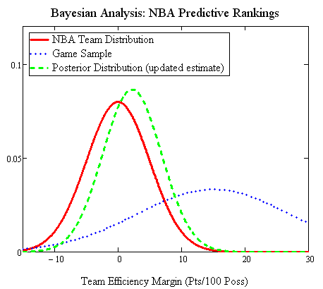
So, with the Bayesian prior (stdev 5, mean 0) and the a first sample, we can get an updated distribution. Of course, to adjust this game for opponent, we must have some idea of how good the opponent is–in this case, I’ll take the adjusted efficiency over the course of this whole season as a reasonable approximation. This game, we’ll assume the actual adjusted efficiency margin for our team was +15–so the distribution has a stdev of 12 and a mean of 15.
Plot it up and we get a posterior distribution:
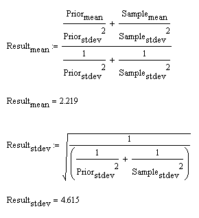
Wait… how did I calculate that? I multiplied the two functions, and scaled it so the sum of the area under the new distribution is still equal to 1. (Yes, that is called calculus.) We can still describe the posterior distribution simply, though, because it’s still a normal distribution: the mean is now 2.22 and the new standard deviation is 4.615.
There is a shortcut–there are formulas to calculate the new mean and the new standard deviation, rather than using calculus and MathCAD to do the work:
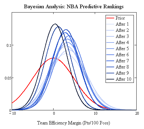
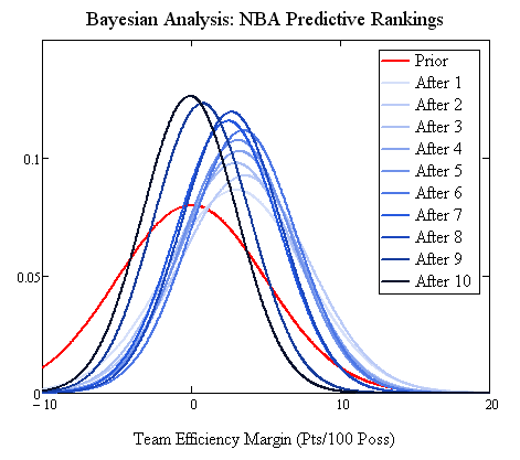
Well, here comes the complex part. We could just keep doing that same thing over-and-over again–but then we’d be weighting all of the games equally, basically just honing in on the regressed year-long-average efficiency differential. That would look like this, for the first 10 games:
But, we had originally intended to look at “predictive” efficiency ratings. So that means we are willing to deprecate older game data somewhat. How much? That really can’t be answered without some empirical analysis.
The basic concept is this: between each game, apply a transformation that increases the standard deviation by a fixed amount. Thus, if the current game has a standard deviation of 12, then the previous game would have a standard deviation of 12 + a, and the next a standard deviation of 12 + 2a, etc… This has the effect of weighting each game 1/(12)^2, then 1/(12+a)^2, then 1/(12+2a)^2, and so on. That can be restated as a weighting of the form b, b-c, b-c^2, b-c^3, etc. In this case, b would be 1/144, and c would be… ugly. (24a + a^2)/[144*(144+24a+a^2)], I believe. Anyway, moving along…
Adding the “penalty factor” depreciates the value of the older samples. The choice of how much depreciation to use requires the empirical work. To do this, I compiled last year’s NBA data and this year’s NBA data, adjusted all of the games for opponent, location, and rest, and set to work. I created a framework using the above methods to create the Bayesian-updated projection for each game, based on the games so far that season.
Finally, I solved for “a”, minimizing the sum of the squared error of the pre-game predictions. The best fit of “a” was 0.20. Going back and checking whether that “12” is correct for the game-level standard error yielded slightly less than 12, but the difference was so insignificant on the overall error (thousandths of 1 percent) that I’ll just use 12.
And so we have a model: the Bayesian prior has mean 0, stdev 5. Each game is set as mean=adjusted performance, standard deviation = 12. Older games have 0.2*n added to their standard deviation, where n is the number of games since that game was played.
Here’s how that looks, for the same 10 games in the graph above (the first 10 games for Atlanta this year, incidentally):
How does that look compared to the previous version without the “penalty”? The distributions are a bit wider and the mean moves a bit further based on more recent data.
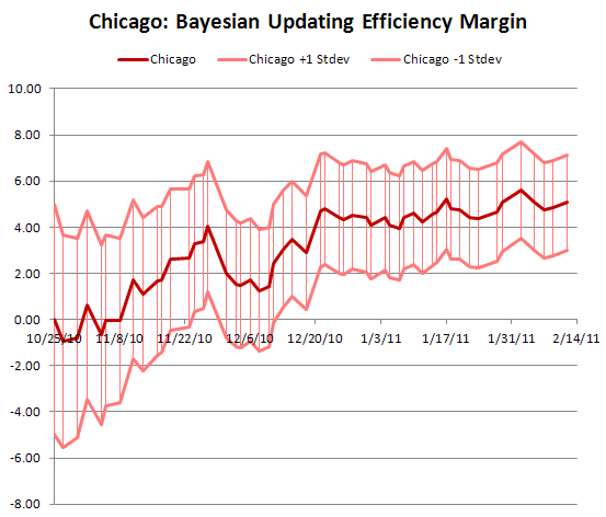
Okay, let’s look at the final product. Here is Chicago through last night:
And here is a look at the current rankings (the errors for all of them are in the 2.05 range–remember, error in this model depends only on quantity of observation, not observed variance of observation):
| Rank | Team | Bayesian Eff. Dif. | Unweighted | Hollinger |
|---|---|---|---|---|
| 1 | MIA | 6.58 | 8.07 | 6.69 |
| 2 | SAS | 6.16 | 7.17 | 7.38 |
| 3 | ORL | 5.19 | 5.68 | 5.88 |
| 4 | LAL | 5.12 | 6.54 | 5.73 |
| 5 | CHI | 5.07 | 5.61 | 5.77 |
| 6 | BOS | 5.05 | 6.93 | 5.47 |
| 7 | PHI | 2.61 | 1.83 | 3.33 |
| 8 | DAL | 2.13 | 3.18 | 4.21 |
| 9 | MEM | 2.08 | 1.78 | 2.01 |
| 10 | NOH | 1.93 | 2.67 | 3.15 |
| 11 | DEN | 1.46 | 2.43 | 1.73 |
| 12 | OKC | 1.37 | 1.45 | 2.32 |
| 13 | POR | 1.07 | 1.11 | 0.53 |
| 14 | HOU | 0.87 | 0.84 | 1.30 |
| 15 | ATL | 0.50 | 1.22 | -1.02 |
| 16 | NYK | 0.25 | 0.51 | -0.51 |
| 17 | IND | 0.04 | -0.27 | 0.60 |
| 18 | PHO | -0.03 | -0.46 | 1.34 |
| 19 | MIL | -0.98 | -1.15 | -1.62 |
| 20 | UTA | -1.66 | -0.31 | -2.40 |
| 21 | CHA | -1.85 | -3.04 | -1.56 |
| 22 | LAC | -2.46 | -2.96 | -3.52 |
| 23 | GSW | -2.54 | -3.10 | -3.35 |
| 24 | SAC | -3.38 | -5.64 | -3.15 |
| 25 | DET | -3.57 | -4.50 | -4.20 |
| 26 | WAS | -4.92 | -6.36 | -6.08 |
| 27 | MIN | -5.02 | -5.91 | -6.13 |
| 28 | TOR | -5.59 | -5.79 | -7.13 |
| 29 | NJN | -5.90 | -6.57 | -6.43 |
| 30 | CLE | -9.53 | -10.96 | -10.32 |
Unweighted indicates a ranking with all games in the season weighted equally. Hollinger comes from today’s Hollinger Power Rankings on ESPN, the primary other power rankings I know of that consider recency effects.
There’s an elite 6 right now, and then… …. Philly, of course!
To truly show how this Bayesian updating method works, here is how each team’s Bayesian efficiency differential has progressed through the year, with one of those lovely Google Motion Charts:
This concludes a remarkably long ramble about Bayesian methods and NBA efficiency ratings. Hopefully the reader has been enlightened, not confused!
I like it. Does changing the value slightly have much effect on prediction accuracy.
Also, just to clarify, you looked at last year’s data and this year’s separately. Nothing from last year influences this year’s predictions – is that correct?
Do you think looking at more years would improve the model or do you converge on the value of a = 0.2 pretty quickly?
Changing either value didn’t change predictive accuracy much, so I don’t think more years will do a whole lot to change things.
When finding the value of 0.2, I looked at each year separately, but regressed as a whole (the models were independent, but I looked for what would minimize the error overall).
That should be “value of a”.
what a bunch a ##…you stats heads think u know it all…there r so many things wrong with this i dont know where to begin…
just kidding, very interesting stuff. A little hard to digest all at once past midnight though!
This is really cool. A little hard to digest, but if I’m understanding correctly your using a Bayesian approach to figure out how well a team is playing “now” (recently). Yes?
So the question is, how well does this model perform? 🙂
Yes, this is the best-fit Bayesian model to predict from the team history in games 1 to N-1 how the team will perform in game N.
How would you like me to measure it? There’s still a ton of variance not explained by the model. Some could be explained by lineup changes, but still there is a ton not accounted for.
I understand there is a lot potentially unaccounted for. Nonetheless, here’s my initial thinking: Start at a reasonable point in the season (10g in? 20g?) and every night, predict the point differential based on Bayesian differential. I think that’s the old Sagarin approach, no? (I’d adjust for HCA and HCA against back-to-backs.) See how many games it gets right and what the errors are. That seems like a simple place to start.
Of course, that might be a complicated place to start because it involves updating the Rankings after every game, but that’s the merit of something like this anyway, so it’s seems less useful to test a “final” ranking against a block of games.
That’s how I did these rankings–hence the motion chart!
Except… how do you adjust for opponent? I used the current non-Bayesian adjusted ratings for the opponent adjustment, and then applied the Bayesian on the already-adjusted game ratings.
Ah right – forgot to activate the flash on that. Really really nice motion chart.
You aren’t following what I’m saying about testing it I think (or maybe you are and I’m about to embarrass myself with simplicity). Let me give you an example using philadelphia. Let’s call t the game number (t=1 is opening night. t=82 the last game of the RS)
At t=18 (dec 3) they are -1.3 when they play the Atlanta Hawks. Atlanta is +1.0. In a linear sense, the expected result is Atlanta to win by 2.3 points. (Again, there might be a better way for those numbers to interact — your math is far ahead of mine.) Atlanta is also playing at home, so they’d need some kind of adjustment (this year on my latest pass it was ~2.5 points — you could estimate the difference per team of course.) So the line should be Atlanta by 4.8 points. Compare that to the final result for a) the difference and b) the W/L result.
(I picked that game at random, and sure enough Atlanta won by 5 points.) Check it around the league every night like that and see how good it is at predicting games. There are plenty of ways to test these things, but that’s the first one that game into my head.
That’s really easy to do. I’ve got all of the data for that; I’ll post the results when I have a chance.
Does the weighing have to be done in the “1/(12)^2, then 1/(12+a)^2” way? I’m currently messing around with 1/(x^b) where b is the number of days this particular game occured before the current date. X has to be determined by CV. Should this lead to the same result, or is your way definitely better?
I guess I’ll try that myself in the next couple of days but figured I might ask anyway
The theoretical weighting for a Bayesian problem should be based on 1/(StdErr)^2.
Commonly, time weighting is done as x^b (not 1/x^b), where b is time period ago and x is less than 1. This implies a specific factor increasing stderr as the time ago increases.
Suppose our x factor is 0.95, so weighting is of the form 0.95^b, where b is time ago.
In a Bayesian standard error formulation, that same weight could be expressed as a standard error of e^(-.5*ln(0.95)) . That makes more sense than increasing the standard error with the 12 + a,2a,… formulation in the article.
My formulation in the article is probably not correct; I should have used something like the ones above.
I recommend using a formulation of x^b, where b is days ago and x<1, found by cross-validation.